Creating a PivotTable with PowerPivot Data

If you see a security warning, click Enable Content. Ensure that the PowerPivot tab is displayed on the ribbon. If you do not see this tab, please complete the steps in the “Enabling PowerPivot” topic first.

Open the PowerPivot window by clicking PowerPivot → Manage:

After a relationship has been created between PowerPivot data, you can create a PivotTable. With the PowerPivot window open, click Home → PivotTable (not the drop-down arrow):

This action will open the Insert Pivot dialog. For this example, ensure that the New Worksheet radio button is selected and click OK:

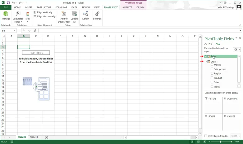
The new PivotTable will now be created in Excel. Inside the PivotTable Fields pane, you will see two sets of fields: Sales and Sheet1. Click on each item to expand them:

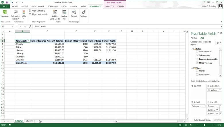
With both sets of fields now expanded, you can see all of the fields that are available. To add a field, simply click its checkbox. For this example, add Salesperson, Expense Account Balance, and Miles Traveled from the Sales field set. From the Sheet1 field set, add Sales and Profit. Now, you can see data from two different sources together in the same PivotTable:

You can work with this PivotTable as you would any other. If you need to access the data in this PivotTable, open the PowerPivot window by clicking PowerPivot → Manage:

If the data in the external source changes, you can refresh the data in the PowerPivot window by clicking Home → Refresh:

Then, you would need to refresh the PivotTable in Excel by clicking PivotTable Tools – Analyze → Refresh.