Multiple Cell References in Microsoft Excel
Excel is capable of completing complex calculations relatively quickly. Most of the time, your calculations in Excel will involve using multiple pieces of data for each calculation. In order to do this, you will need to be able to reference multiple cells at the same time.
For more on MS Excel training classes in Los Angeles call us on 888.815.0604.
Using Multiple Cell References
Consider the sample worksheet below:
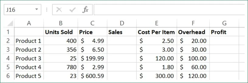
In order to calculate profit per product, total sales figures need to be calculated and then the cost of the items needs to be subtracted from the sales. To calculate the sales amount, select cell D2 and type =B2*C2 in the formula bar:
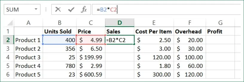
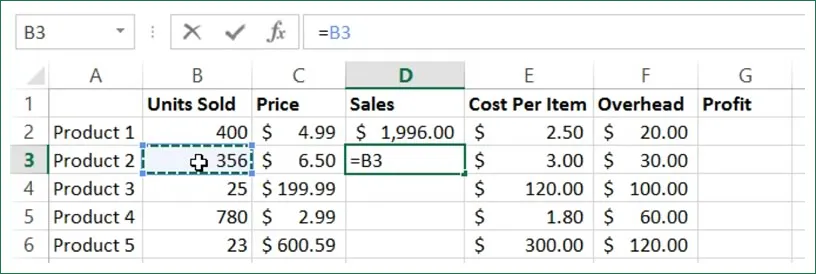
Press Enter. Next, select cell D3 and click inside the formula bar. Type an equals sign (=) to begin the formula and then click cell B3:
With B3 now inserted into the formula, you now need to add a mathematical operator. Type * for multiplication and then click C3 to add that cell to the formula:
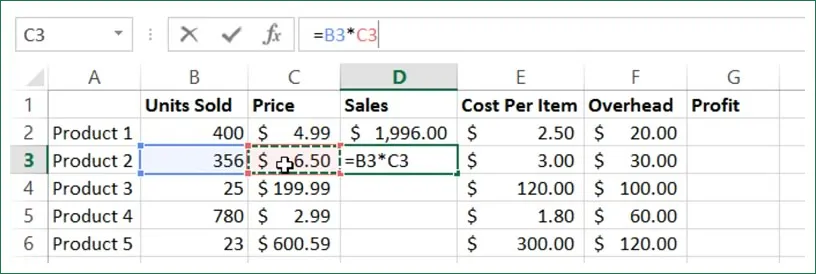
Press Enter to complete the formula
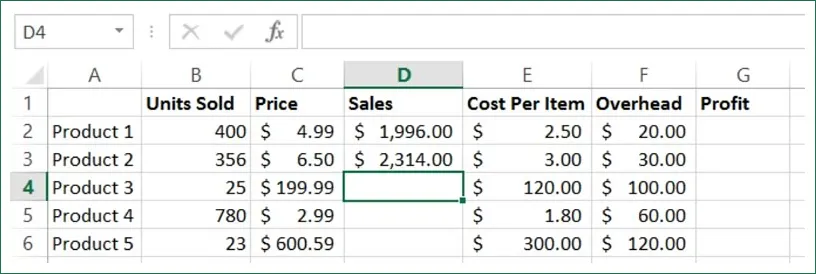
Now that the sales values have been calculated for these two products, you need to calculate the profit. Profit is calculated by subtracting the expenses from the sales. Keeping the order of operations in mind, the formula will be: Sales - (Units Sold * Cost Per Item + Overhead).
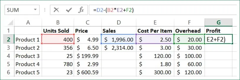
Click inside cell G2 and then type the following formula: =D2-(B2*E2+F2). Note that each cell will be color coded as it is entered into the formula:
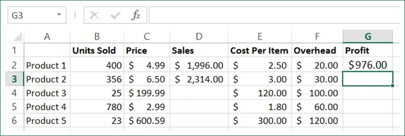
Press Enter. You will now see a calculation of the profit for the first product:
Save the changes that you have made to the current workbook and close Microsoft Excel 2013.
Using 3D References
A reference that refers to the same cell or range of cells on multiple sheets is called a 3D reference. They are useful when referencing several worksheets that follow the same pattern. For example, 3D references could become handy when you consolidate different sales results from different departments, for example.
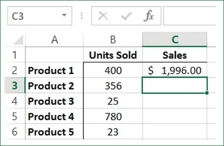
In the sample workbook, the data you need for a particular formula is spread out over two worksheets. With Sheet1 open, click cell C2 and then click inside the formula bar. Type =SUM(Sheet2!B2*Sheet1!B2):
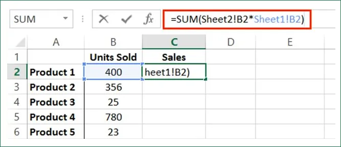
As you can see, “Sheet2!B2” references data in cell B2 on Sheet2 in the current workbook, while Sheet1!B2 references data in cell B2 on Sheet1.
Press Enter to apply the new formula. You will see the results displayed:
Save the changes that you have made to the current workbook and close Microsoft Excel 2013.
